tadamichi
What is driving this stock market melt-up that is not underpinned by extraordinarily strong fiscal flows and runs in the face of the usual seasonal patterns?
The table below shows the US sectoral balances up to the last month. The information is prepared from the US national accounts.
US Treasury and Author calculations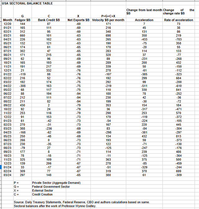
In March 2024, the private sector recorded a surplus of $380B and this is a very positive result for asset markets as financial balances in the private sector have risen and caused the aggregate demand for goods, services, and investment assets to grow.
From the table, one can see that the $380 billion private sector funds surplus came from a $297 billion injection of funds by the federal government (and this includes the new injection channel from the Fed of around $8B from interest on reserves that went directly into the banking sector), less the -$65B billion that flowed out of the private domestic sector and into foreign bank accounts at the Fed (the external sector X) in return for imported goods and services. Bank credit creation added $148B, which is over double last month’s rate.
The numbers for the last six months or so are nothing special like during the COVID emergency spending back in 2020 shown at the beginning of the table and where a steep stock market recovery took place. The fiscal flows alone cannot explain the steep, sustained melt-up in the US stock market.
The table below shows how much money the federal government took out of their bank account at the Federal Reserve. When the government spends money, it gives more money to the private sector and helps the stock market go up.
US Treasury and Author calculations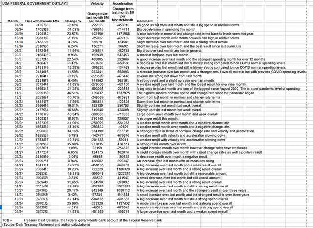
The table shows that total outlays were nearly half a trillion down over the previous month and in the region of $2.5T. This month Federal taxes, fees, charges, and bond turnover allowed $297B of that spending to remain in the private sector and form the federal deficit which is dollar for dollar the private sector surplus. When one deducts the current account deficit from this result, the private domestic sector balance is $228B. In terms of purchasing power, this improves again when one adds the $148B of bank credit creation.
Though a strong result, it is not so strong that it explains the stock market strength that has taken place over the last six months.
The chart below shows how the rise and fall of the US private-domestic sector balance tends to lead the SPX.
US Treasury and Author calculations and SPX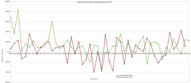
Last month the lead of the private domestic sector balance over the (SPX) predicted that the (SPX) would finish March higher than it began and this did indeed happen.
This month the chart is predicting the same result for April given the continued strength of the private domestic sector fiscal flows. So far, this has been the case and is likely to continue.
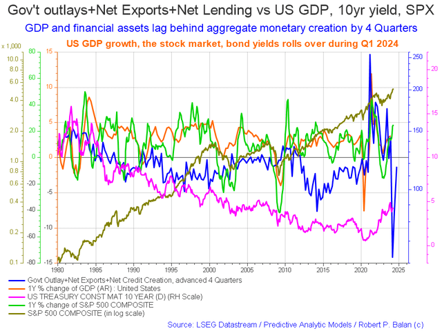
The chart below shows how the information in the US sectoral balances table is changing over time, taking into account any delays in the impact of these changes. This is like a tool that helps us see what’s happening in the market from far away.
The blue line represents the money that the government spends and the credit that banks create, minus the current account balance. It can predict economic changes up to four quarters in advance.
The change over last month is that the SPX has risen, as has GDP and bond yields. The leading blue line continues to rise.
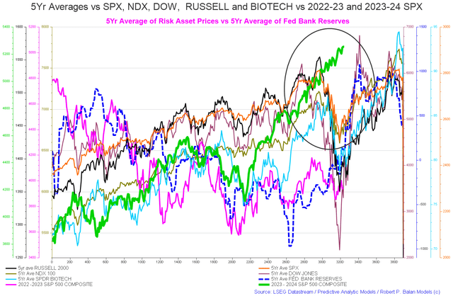
The chart below shows the five-year average of the seasonal stock market patterns for the SPX (SPX), Nasdaq (NDX), Dow (DIA), Russell 2000 (RTY), and Biotech market indexes. The black oval shows where we are now.
This chart shows clearly how the green line has ignored the expected seasonal pattern set by the orange line. The orange line is the five-year average of the SPX. True to form, the SPX should have dipped into the end of the first quarter of 2024 and allowed for a buy-the-dip opportunity. There should have been at least two opportunities to buy seasonal dips this year, and they have not occurred, and one begins to ask why.
Four factors come to mind:
1. Treasury interest income from higher interest rates.
2. Global fiscal spending by world governments.
3. The coming peak in the real estate cycle.
4. Interest on reserve balances paid to banks by the Federal Reserve Banks rising with interest rates.
These factors will be discussed in more detail below.
1. Treasury interest income:
One major thing that is very different over the last 18 months or so is the position of the Fed and its interest rate policy.
What is different from other years is that we now have high-interest rates, and it could be solely the treasury income boost going to wealthy recipients who then buy paper assets in a narrow focused way out of scale with normal asset buying patterns.
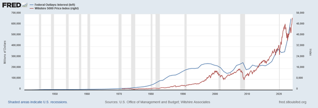
The chart below shows a very long-range and broad growth relationship between federal interest outlays and the stock market.
It would appear that federal outlays for interest lead the stock market by several quarters and that as the stock of treasuries has grown the effect has accelerated and the curve has become steeper as time has gone on. The curve is nearly vertical now.
2. The confluence and rise of the lagged effect of the G5 fiscal flows.
The G5 flows are the sum of the spending of the largest five economies in the world. The C5 are the balance sheets of the five largest central banks in the world.
Mr. Robert P Balan of the Predictive Analytic Models Investment Service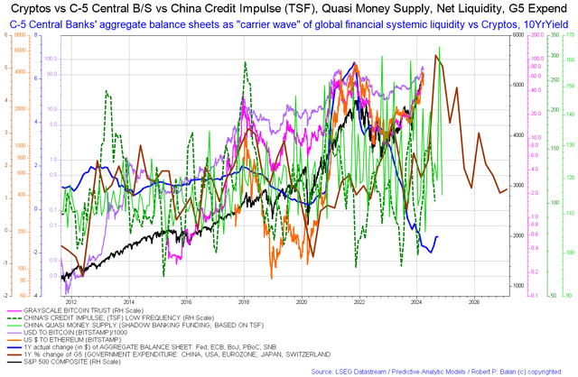
Together, the G5 and C5 fiscal flow impact what is known in fluid dynamics as a carrier wave upon which all other fiscal flows and market effects are based.
The above chart shows that the brown carrier wave is rising steeply into 2024 and this will tend to lift asset markets with it.
The brown line on the chart above shows this carrier wave. The next chart shows this in a more granular format but does not go as far as the chart above.
Mr. Robert P Balan of the Predictive Analytic Models Investment Service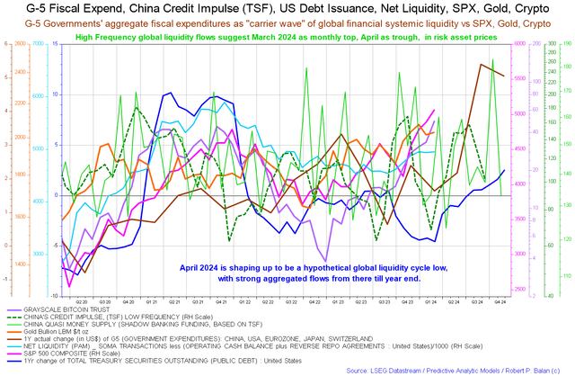
The nearer-term view of the same information shows how the brown line dips into the first quarter of this year and then rises from the second quarter onward.
These charts are not very granular, and it could be that the macro uplift from the G5 flow has arrived earlier than forecast and would explain the unusual buoyancy in the markets. It also points to the fact that things are likely to get better rather than worse as the year rolls on.
3. The economic rent effect from the last mania-driven winners curse phase of the real estate cycle.
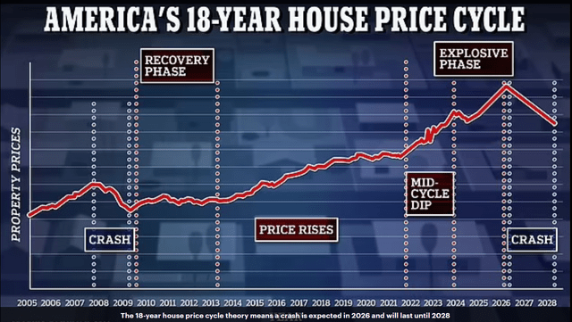
The chart above shows the course of the real estate cycle and how it is now entering into its last and most explosive and speculative stage. Rising property prices create a focused wealth effect among property owners and are the culmination of price rises since the recovery began in 2009. 15 years of land price growth reaching its peak, getting monetized, and then entering asset markets.
Land prices rise and culminate so much that there is a wealth effect starting based on the asset value of normal people’s homes. Some of them would then get a home equity loan that enables the wealth that has grown out of nowhere to be monetized and spent on paper assets, further driving a stock market melt-up in a focused way. There you see how land price rises drive credit creation and thus aggregate demand even for normal people and not just the big end of town, and this money finds its way into the stock market in a focused way.
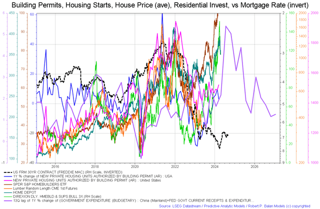
It’s important to check the housing market regularly because it’s closely related to the overall economy, and it’s expected to reach its highest point in 2026.
The chart shows aspects of the housing market. In this instance, we have the price of lumber (orange line and that tends to rise in a boom) appearing to bottom and be close to a local low and still not rising. Now all falling month over month are the home-builder ETF, Home Depot. Housing starts and permits rose nonetheless. The Freddie Mac 30-year contract rate fell [which is normally good for housing and may explain why permits and approval increased at the same time as more people took on a slightly cheaper loan and chose to build or buy] Important to note though is the purple government expenditure line rising through most of the rest of 2024 before dropping and rising again into 2025. This line is the same fiscal carrier wave that sets the overall trend for all other waves that follow in its wake, and is shown at point two above.
4. Interest of Reserve Balances at the Fed
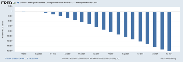
Another important factor is the interest on reserve balance income that is flowing directly to banks as a result of high-interest rates, and is related to the first factor listed above. This is shown in the chart below
Banks tend to deploy spare income into income-yielding paper assets such as stocks and bonds at the rate of about $10B per month.
The 4 Way Financial Venturi Effect.
The four factors described above support the thought experiment that the current and continuing stock market melt-up in the face of only average fiscal flows are driven by a financial Venturi Effect.
Wikipedia
The treasury interest income, IORB, and monetized wealth from the real estate cycle are income sources where the recipient is largely already wealthy. In the search for yield and a high level of discretionary spending, the recipient seeks to invest this money into paper assets and thus creates an out-of-scale stock market rally in comparison to the actual strength of the current fiscal flows.
The background effect of the overall rise in the lagged impact of the G5 fiscal flows underpins and reinforces this Venturi effect.

